The aim of this tool is to study the influence of the communication BANDwidth and the communication LAtency for an MPI application. In French “and “ is translated by “et”. In this language Bandela is exactly read as “BAND et LA”. Bandela sounds like the name of a Latin song so we like it.

How does Bandela work

Bandela works in 2 steps.

Step 1

Dynamically linked with a special Mpi library, a run of the application, on a window of interest, has to be executed in order to instrument it. Some libmpi internal kernels (more about them appears below) are catch and a record is created for each instance of them with the following information:

- Sender and receiver ranks

- main function ( mpi_bcast, mpi_reduce,….), kernel activated (isend, irecv…), MPI communicator,

- size of the transfer request, Data type (is it a “symmetric”, i.e. data may be transferred using single copy), Tag,..

- The computational time since the previous Mpi call. No MPI timing at all are taken.

Step 2

All the computation timings gathered in step 1 are “replayed” and a model is applied for communication. The name of the program, which implements the model, is replaympi.

On output this process produces some detailed and accurate information about the Mpi communications of the application.

The advantages of using a model for this kind of studies are:

Any “real time” tool for studying such phenomena have to find a balance between the amount/quality of data collected and the overhead to get such information. A model have no such constrains. As we don’t record any communication timings we don’t care to perturb them.

Any “real time” tool just reflects what it is. It cannot answer the question: “What if”:

-Transfer bandwidth increased or decreased.

-Latency (but we need to precise what does that means) increased or decreased.

One can figure out what is about with a different hardware.

A detailed MPI_BCAST example:

Consider a run on 4 CPU for the following Fortran program which performs a single MPI_Bcast . The arrivals to this mpi_bcast() collective routine occur in the rank order:

program test_bcast

include 'mpif.h'

parameter (isz=1000 )

parameter (n_loop=1)

dimension array(isz,isz)

common /ttt/array

call mpi_init(ierr)

call mpi_comm_rank(mpi_comm_world,myrank,ierr)

call mpi_comm_size(mpi_comm_world,nprocs,ierr)

idest=myrank+1

if (idest.eq.nprocs)idest=0

isrc=myrank-1

if (isrc.eq.-1)isrc=nprocs-1

C Just some dumb computation to have ranks to call mpi_bcast

C in the rank order with a big delay between arrivals

do n_l=1,n_loop

do i=1,2*(myrank+1)

do j=l+1,(isz/nprocs)*(myrank+1)

do k=2,isz

array(1,j)=array(1,j)+array(k,j)

enddo

call MPI_bcast(array(1,1),isz*10,

1 MPI_REAL,nprocs-1,MPI_COMM_WORLD,ierr)

enddo

call mpi_finalize(ierr)

end

On Altix using the SGI MPT MPI library execute the following commands:

f77 –o test_bcast test_bcast.f –lmpi

setenv LD_LIBRARY_PATH BANDELA_ROOT/1009/mpt_lib:${LD_LIBRARY_PATH}

setenv MPI_BUFFER_MAX 2000

mpirun –np 4 BANDELA_ROOT/bin/bl ./test_bcast

Four files corresponding to the 4 MPI threads will be created: bandela.0, bandela.1, bandela.2, bandela.3

For example bandela.0 when formatted looks like:

Rank	Main function	Active Kernel	Dest or source	comm	tag	count	datatype	request	Comput time
0	init	init	-	-	-	0	0	-	0.000443
0	bcast	isend	2	1	-3	1	12	0	0.119647
0	bcast	wait	-	-	-	1	0	0	0.000002
0	bcast	isend	1	1	-3	1	12	0	0.000001
0	bcast	wait	-	-	-	1	0	0	0.000000
0	bcast	irecv	1	1	-12	1	3	1	0.000014
0	bcast	wait	-	-	-	1	0	1	0.000001
0	bcast	irecv	2	1	-12	1	3	1	0.000004
0	bcast	wait	-	-	-	1	0	1	0.000001
0	bcast	isend	2	1	-3	1	3	0	0.000002
0	bcast	wait	-	-	-	1	0	0	0.000001
0	bcast	isend	1	1	-3	1	3	0	0.000001
0	bcast	wait	-	_	-	1	0	0	0.000000
-1	bcast	irecv	3	1	-3	10000	14	1	0.000001
0	bcast	wait	-	-	-	1	0	1	0.000001
0	finalize	finalize	-	-	-	0	0	-	0.000008

The –1 =–(rank 0 –1) on record 10 means that the receive buffer is symmetric. This has no consequence here for an irecv but for an isend such transfer may be done single copy.

This is the sequence of the elementary calls the Mpi library has generated to handle the Mpi_bcast for Mpi rank 0. On SGI MPT these elementary internal libmpi routines are: MPI_SGI_BARRIER,MPI_SGI_request_send, MPI_SGI_request_recv, MPI_SGI_request_test, MPI_SGI_request_wait (this last call actually MPI_SGI_request_test but only one wait record is created for a wait request;).

These 5 routines are conceptually equivalent and use the same parameter semantic than, respectively, mpi_barrier, mpi_irecv, mpi_isend, mpi_test, mpi_wait. All mpi requests are transformed into a sequence of the above routines (the few exceptions are taken into account). These routines are the only ones to be modeled. The Intel/MPICH2 library doesn’t take always these same simple ways but the tracing routines manage to finally generate traces compatible with this simple model.

Replaympi the model, How does it work?

Suppose we would have to retrieve the communication time for the following MPI sequence modeling a run on a single Altix host. Note that the only information we have is:

-The computation time,

-The destination or source of the request

-The count and data type of the request

-An ” average” transfer bandwidth and an average latency. Say 700 Mb/s and 2 micro seconds an Altix :

| : computation outside MPI, the time recorded.

x: wait for data to be sent or received

Time	Rank 0	Rank 1	Rank 2
0	\|	\|	\|
1	computation	computation	computation
2	\|	\|	\|
3	Isend to 1 req. 1	\|	\|
4	\|	\|	Irecv from 2 req 1
5	\|	Isend to 2 req 1
6	\|	\|	Physical Transfer 1->2
7	\|	\|	Wait req1
8	Wait req 1	\|	\|
9	x	\|	finalize
	x	\|
	x	\|
10	\|	Irecv from 0 req 2
11	\|	Wait req 1
12	\|	Wait req 2
13	\|	finalize
14	finalize

The model always treats the mpi event occurring the first. I.e. the record for a rank not locked having the minimum for :

Comput_time + comm_time + time_in_record for rank.

This minimum is the real time clock to consider.

So in time order:

rank 0 comes real time =3, some software latency is added to comm_time for rank 0

Then rank 2 comes real time =4 , some software latency is added to comm_time for ranks 2

Then rank 1 comes real time =5 , some software latency is added to comm _time for rank 1. As a consequence of this event some transfer time is added to comm _time for rank 2

Then rank 2 comes real time=7, some software latency is added to comm_time for 2

Then rank O comes real time =8, rank 0 is stuck

Then rank 2 terminates

Then rank 1 comes real time=10, some software latency is added to comm_time for rank 2, the transfer time is also added and the real time clock is updated accordingly. As a consequence of this event, comm 0 is synchronized comm_time for rank 0 = real time -comput time 0. Rank 0 is unstuck

Etc, etc

By applying this technique to the small Fortran program above the model gives the following output where everything before the “==” is input to the model. The input values will be discussed latter in this document. The set of bandela.xx files are of course also inputs to the model.

NUMBER_OF_HOSTS 1

HOST_TYPE 0

mpi_buffer_max 2000

INTRA_HOST_BANDWIDTH_PEAK 800.00

INTRA_HOST_LATENCY 2.00

INTRA_HOST_BARRIER_LATENCY 10.00

BLOCK_HOST 0

NUMBER_OF_PROCS 4

MPI_RANKS 0-3

ADAPTERS 0

=====================================================

CPU 0 Total Time : 0.465109 s

CPU 0 Total computation Time : 0.019306 s

CPU 0 Total communication Time : 0.445803 s, Wait : 0.445753 s

CPU 0 latency: 0.000050 s, mess<=1024: 0.000000 s, mess>1024: 0.000000 s

CPU 0 Bytes(Mb) : recv 0.000000 buffered 0.000000

=====================================================

CPU 1 Total Time : 0.465163 s

CPU 1 Total computation Time : 0.126103 s

CPU 1 Total communication Time : 0.339059 s, Wait : 0.338529 s

CPU 1 latency: 0.000030 s, mess<=1024: 0.000000 s, mess>1024: 0.000500 s

CPU 1 Bytes(Mb) : recv 0.400000 buffered 0.000000

=====================================================

CPU 2 Total Time : 0.489037 s

CPU 2 Total computation Time : 0.249799 s

CPU 2 Total communication Time : 0.239238 s, Wait : 0.238688 s

CPU 2 latency: 0.000050 s, mess<=1024: 0.000000 s, mess>1024: 0.000500 s

CPU 2 Bytes(Mb) : recv 0.400000 buffered 0.000000

=====================================================

CPU 3 Total Time : 0.489039 s

CPU 3 Total computation Time : 0.488519 s

CPU 3 Total communication Time : 0.000520 s, Wait : 0.000000 s

CPU 3 latency: 0.000020 s, mess<=1024: 0.000000 s, mess>1024: 0.000500 s

CPU 3 Bytes(Mb) : recv 0.400000 buffered 0.000000

=====================================================

Wait: The time the CPU was not in the Mpi library nor waiting for the completion of a physically started transfer. This is the time the CPU cannot do anything but wait for g but wait for another CPU to post a message.

Latency: The time accounting to the Hardware/MPI library latency. The model add the latency(0) time to any send/receive internal transfer. On a single host this here this time is exactly equal to number of requests * Latency(0)

Transfers: The time the communication engine was busy transferring on this CPU. This time is itself spilt into small transfers (inferior to 1024 bytes) and big transfers (superior to 1024).

Using Bandela

Instrumentation

To capture the information necessary to the model a run of the application with the targeted number of CPU must be done. In most cases no recompiling nor relinking is necessary.

On Altix with the SGI MPT library

setenv LD_LIBRARY_PATH BANDELA_ROOT/1009/acquire:${LD_LIBRAY_PATH}

mpirun –np <nb_CPU> BANDELA_ROOT/bin/bl <your_mpi_binary your_arguments>

With Intel/MPICH2 library

setenv LD_LIBRARY_PATH \

BANDELA_ROOT/1009/acquire_intel:${LD_LIBRAY_PATH}

setenv I_MPI_DEVICE shm

mpiexec –np <nb_CPU> BANDELA_ROOT/bin/bl <your_mpi_binary your_arguments>

Whatever the Bandela library used, it may happen the launcher (BANDELA_ROOT/bin/bl) failed to launch your application. In such case a relink with the libbandela.so or libbandela.a is necessary. Then run simply:

mpirun/mpiexec –np <nb_CPU> <your_mpi_binary your_arguments>

Note that the language used by the application(Fortran or C) doesn’t matter.

Full instrumentation

Data is collected starting at mpi_init and ending at mpi_finalize. Nothing more that what describe above is necessary.

Partial instrumentation

In order to select a window of observation (to skip the initialization time for example) Bandela provides 2 mechanisms.

Inside the application:

Fortran:

Call bandela_start()

Call bandela_ends()

Bandela_start_();

Bandela_end_();

The BANDELA_PARTIAL_EXPERIMENT variable must also set to “YES” in order to instruct the Bandela library to delay experiment up to the bandela_start() call.

This is the responsibility to the user to ensure that these routines are called by ALL the MPI threads.

Outside the application

Bandela will count the calls to some selected MPI collective routines with some selected MPI communicator and starts and ends according to the values of some environment variables. In addition setting BANDELA_SHOW_W will print a explicit message to “ stdout” after each call to the watched routine. This allows the user to match the window of observation with the application prints on “stdout”. See man_libbandela.txt for more detail on these environment variables.

Example:

# watch MPI_Bcast with MPI_COMM_WORLD (the default communicator)

# and print a message each 10 calls

setenv BANDELA_WATCH_ROUT MPIBCAST

setenv BANDELA_SHOW_W 10

# set a “infinite” window as we don’t know the right one yet

setenv BANDELA_BARRIER_START 0

setenv BANDELAçBARRIER_ENDS 1000000000

Supposing calls to MPI_Bcsat 200 to 1000 is a good choice

setenv BANDELA_WATCH_ROUT MPIBCAST

setenv BANDELA_BARRIER_START 200

setenv BANDELA_BARRIER_ENDS 1000

Modeling the communications

Inputs to the model

The model (BANDELA_ROOT/replay/replaympi with SGI MPT BANDELA_ROOT/replay_intel/replaympi with Intel/MPICH2) must be run in the directory where the bandela.xx are located.

An input on “stdin” (replaympi <input ) must also be provided with the following format:

Any line starting with the ‘#’ character is a comment.

A line always starts with a keyword.

An upper case keyword must always appear in the input

A lower case keyword is optional:

The list a keywords follows:

NUMBER_OF_HOSTS <integer value>

HOST_TYPE <0|1|2>

synchronous <Y|N>

cpu_boost <real value>

block_max_ignore_collective

ignore_safely

ignore_index

block_max_calipers

calipers_boots

mpi_buffer_max <integer value>

small_message_size <integer value>

adapter_select <0|1>

local_bandwidth <real value>

INTRA_HOST_LATENCY

INTRA_HOST_BANDWIDTH_PEAK

INTRA_HOST_GET_PUT_LATENCY

INTRA_HOST_GET_BANDWIDTH_PEAK

INTER_HOST_LATENCY

INTER_HOST_BANDWIDTH_PEAKS

< 2 real values in MB/s>

inter_host_degradation_ratio

block_points <integer values>

sizes <block_points <integer size>

values <block_points <real values>

INTRA_HOST_BARRIER_LATENCY

INTER_HOST_BARRIER_LATENCY

inter_host_long_latency <real value>

intra_host_long_latency <real value>

delay_for_long_latency <real_value>

BLOCK_HOST <integer value>

NUMBER_OF_PROCS< integer value>

MPI_RANKS <list>

ADAPTERS <integer value>

First non comment line in the input

Type of cluster topology

For an inter host transfer on MPT or “shm” device with Intel/MPICH2, the CPU is blocked till the end of the transfer(synchronous=Y) this is the default. This simply because the transfer are done by CPU on shared memory and so the CPU cannot do anything else. On some RDMA devices the CPU may be free to compute while the RDMA does the transfer in parallel. Setting the “synchronous to N allows to model such behavior.

All CPU time are divide by this value. Default is 1.0

These 3 parameters allow the model to compute timings as if some MPI collective functions were not present(see latter in this document)

These 2 keywords allow the model to predict the global execution time with some computation optimization on some particular area of the application as opposed to the “cpu_boots” keywords that lead to apply a computation optimization everywhere to any (see latter in this document)

The same meaning as the MPI_BUFFER_MAX env. Variable. Default is 1048575. Only meaning full for SGI MPT.

The size in Bytes of what must be considered as small message. It does not change any computation it just change how the times are split between short and long messages

Default is 1024 Bytes

0 round robin, 1 first free (not implemented yet)

default is 0

The Bandwidth (MB/s)for local (buffering) copies. Default is 2 time the Intra host peak Bandwidth

These seven keywords described

The cluster performance.

Each of them can be optionally followed by the block of keywords described below. These 3 keywords detail the performances in regard to the transfer size.

INTER definition are only legal and necessary if more than one host is defined.

INTRA_HOST_GET_PUT_LATENCY and INTRA_HOST_GET_BANDWIDTH_PEAK are only necessary if an mpi_get or mpi_put are in traces. Note that half of the speed will be applied for an MPI_Put

These 3 keywords are optional

For the keywords just above. They always comes together with the same units as above

For the SGI MPT library this is the Barrier latency to apply. If the communicator implies Intra host communication only INTRA_HOST_BARRIER_LATENCY is used. If the communication implies an inter host echange the INTER_HOTS_BARRIER_LATENCY is used. The Intel/MPICH2 library handles barriers through regular send/recv/wait kernels. In this case setting this keyword leads the model to ignore such send/recv/wait kernel generated for the barrier and to apply latency times the same way it does for MPT. This will only work if the traces were taken with the BANDELA_FAST_BARRIER_RECORD environment variable set.

All values are times in micro seconds. When running with a TCP device, if the request waits for too long on the socket the process is disconnected from the CPU by the operating system. In such case the effective latency become far bigger that the one that can be measured with a Ping-pong test (hundred of micro seconds instead of dozen of micro seconds). If these keyword are set the model will apply long_latency if the arrivals for a send/recv pair are bigger than delay_for_long_latency

1 BLOCK_HOST per host must be defined. At least one host must be defined

Model input examples

Host type 0 (single host)

This is a single host type.

-Using SGI MPT Symmetric data are sent single copy depending of MPI_BUFFER_MAX

-The receiving CPU does the transfer

A simple input to model an Altix system with 8 CPU using the MPT corresponding to the above figure follows.

NUMBER_OF_HOSTS 1

HOST_TYPE 0

mpi_buffer_max 2048

# average Mpi bandwidth is 700MB/s

INTRA_HOST_BANDWIDTH_PEAK 700.00

# average latency is 2 micro second for a send-recveive

INTRA_HOST_LATENCY 2.0

#intra host barrier latency is 10 micro second

INTRA_HOST_BARRIER_LATENCY 10.00

# this is a single host no adapter connection

BLOCK_HOST 0

NUMBER_OF_PROCS 8

MPI_RANKS 0-7

ADAPTERS 0

The same input on the same machine but when using the Intel/Mpich2 library:

NUMBER_OF_HOSTS 1

HOST_TYPE 0

#mpi_buffer_max 2048 no meaning with the Intel library

INTRA_HOST_BANDWIDTH_PEAK 600.00

INTRA_HOST_LATENCY 4.0

#INTRA_HOST_BARRIER_LATENCY 10.00 no meaning

BLOCK_HOST 0

NUMBER_OF_PROCS 8

MPI_RANKS 0-7

ADAPTERS 0

Note that the traces collected with the Mpt library (directory 1009/acquire) must be processed with the 1009/replay/replaympi model while the traces collected with the Intel/Mpich2 library (directory 1009/acquire_intel) must be processed with the 1009/replay_intel/replaympi model. But the input above for the Intel library can be applied to traces got with the MPT library (in order to model what would be the performance drop using the Intel library instead of the MPT one) and the other way round.

A more sophisticated input to model a 256 CPU Altix system follows. It defines a Bandwidth/ latency function depending of the transfer size.

NUMBER_OF_HOSTS 1

HOST_TYPE 0

mpi_buffer_max 1048576

cpu_boost 1.0

INTRA_HOST_LATENCY 2.

block_points 5

sizes 64 512 1024 2048

values 2.15 4.3 5. 6.

INTRA_HOST_BANDWIDTH_PEAK 800.

block_points 2

sizes 4096 8192

values 400. 600.

INTRA_HOST_BARRIER_LATENCY 10.

BLOCK_HOST 0

NUMBER_OF_PROCS 256

MPI_RANKS 0-255

ADAPTERS 0

It must be understood that specifying the Mpi performance using Latency or Bandwidth is strictly equivalent. To a latency corresponds a bandwidth = req_size/(latency-latency(0)). Simply, for small transfers, a latency is more meaningful and a Bandwidth is more meaningful for a big transfer.

Cluster type 1 (said Numaflex)

Cluster type 1 is said Numaflex because it was developed especially for JP Panzierra who needed a very sophisticated model of the SGI Numaflex architecture. An API was developed for this purpose.

Cluster type 1 can model the same Numaflex single image topology such as SGI O3000 or Altix running XPMEM (performance on an Altix partitioned machine is the same than the equivalent single image Altix with XPMEM) than Cluster type 0 but it is not restricted to that. It also allows to describe some other topology. In that case it will be up to the developer of the library to define or read an input for such topology, for example the JP Panziera library uses a set of environment variables for such purpose

In any case the topology must follow the following rules:

Transfer is synchronous and not interleaved. The Mpi_isend function will be locally buffered depending of some criteria such as the request size, MPI_BUFFER_MAX variable, etc.

Only the receiving physical transfer is computed but the host library.

The standard input to Bandela must be a single host input. The INTRA bandwidth definition must be present and is used to evaluate local buffering if any. The host model only takes care of receiving.

Cluster type 1 API:

The user must provide 4 routines gathered in a dynamic library libtopo.so. It must also set the LD_LIBRARY_PATH environment variable to point on the location of this library prior to call the model. It must call replaympinuma instead of replaympi.

#include "BANDELA_ROOY/include/REPLAY/numa_interface.h"

void numaflex_start(int nprocs, double buffered_bandwidth);

Called at the start of replaympi. The buffered_bandwidth is passed but the developer of a libtopo.so can do what he wants with this information. The real time is implicitly zero here.

void numaflex_end(double real_time);

Called at the end of replaympi. The real_time variable gives the real time at the end.

double compute_bandwidth_for_arrival(double real_time,

int receiver,int sender,int req_size, int nb_live,

bandela_item *interface_array);

void compute_bandwidth_for_departure(double real_time,

int receiver,int sender,int nb_live,

bandela_item *interface_array)

compute_bandwidth_for_arrival signals the start of a new transfer issued by receiver to get req_size bytes of data from sender.

compute_bandwidth_for_departure signals the completion of the transfer previously issued by receiver to get data from sender.

In both cases nb_live gives the number of valid entries in array interface_array, each entry representing a transfer requests :

-Already running ( compute_bandwidth_for_arrival )

-Still running(compute_bandwidth_for_departure ).

In addition, the entry interface_array[nb_live+1] must be fill with the new arrival bandwidth and conveniences ( if any) (compute_bandwidth_for_arrival).

The format of a bandela item defined in numa_interface.h:

typedef struct bandela_item_ {

int func; // Bandela internal usage

int receiver;

int sender;

double old_bandwidth;

double new_bandwidth;

void *convenience ; /* these pointer can be set or not

by the host model, Bandela will

maintain the association

with the transfer item

} bandela_item ;

compute_bandwidth_for_arrival returns the bandwidth given to the new request and it updates the interface_array with the new bandwidths for the other lived requests

compute_bandwidth_for_departure updates the interface_array with the new bandwidths for the still lived requests.

Existing libtopo.so libraries:

A library written by JP Panziera modeling very precisely several Numaflex architectures (O2000, 03000, Atix3000, Altix 350) is available) in BANDELA_ROOT/1009/replay/JPPFLEX/libtopo.so

This library is driven by a set of environment variables. You can run a first time replympinuma to get a documentation of such variables

Cluster type 2 (switch)

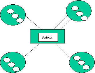
With this type of cluster, each host is a shared memory machine like the Altix. All the hosts are linked to the switch. At least one link to the switch must be present but the numbers of links are not necessary equals.

All the adapters/cards to the switch are equivalent meaning that all the bandwidths definitions over one link are equals. All the hosts CPUs are equivalent but the number of CPUs are not necessarily equals

Each host works as a type 0 host.

The switch is perfect. This means that the link performance only depends on itself. For example, for a send from rank_A to rank_B, the model works this way:

Data have to be fully buffered into the switch by some adapter/card with a performance which only depends on what rank_A previously requested to the adapter(in or out). Then, when things have been fully buffered on the switch, rank_B can start the receiving process. Rank_B depends on rank_A because it has to wait that rank_A terminates this particular send. But the performance of link B doesn’t depend of the activity on link A. Because of this 2 steps, when we usually say, for example, that a send/receive performs at say 240 Mb/s, this bandwidth include the buffering in the switch and the read from the switch. So bandwidths have to be considered doubled by the model (480 Mb/s for this example) in regard to the input definition which has to be set accordingly as what could have gotten by a Ping-Pong test. I.e. 240 MB/s in this example.

The Inter host transfer can be or not “synchronous”. The Mpt Infiniband support is, for example, currently synchronous. It may be asynchronous in the future. Synchronous means that a CPU is locked waiting for the transfer request to complete. With an hardware such the Infiniband this is not necessary. The CPU may fire the transfer and return to the user. The Infiniband RDMA doing the transfer in parallel. The CPU in this last case would only be locked if an mpi_wait for the associated transfer is not completed. Note that we don’t know a lot of applications that could get advantage of such asynchronous feature even when such applications are written with this asynchronous transfer in mind. Anyway Bandela can model it.

The Inter host transfer can or not “interleaves” the requests. A synchronous CPU (say CPU_A) cannot interleave anything, but an other (say CPU_B) may use the shared adapter/card. When not interleaved CPU_B must wait. If interleaved CPU_B shares the adapter/card bandwidth with CPU_A. The default is interleave=Y.

An example of Bandela input for a Cluster of Altix follows.

# CLUSTER of 3 Altix 32x32x16

# 2 IB card on the 32 CPU machines 1 on the 16 CPU machine

NUMBER_OF_HOSTS 3

HOST_TYPE 2

mpi_buffer_max 1048576

cpu_boost 1.0

# current Mpt Infini band implemetation

# is synchronous and interleave

synchronous Y

# card select is round robin

adapter_select 0

INTRA_HOST_LATENCY 2.

block_points 5

sizes 64 128 512 1024 2048

values 2.15 4.3 5. 6. 7.5

INTRA_HOST_BANDWIDTH_PEAK 800.

block_points 2

sizes 4096 8192

values 400. 600.

INTRA_HOST_BARRIER_LATENCY 10.

INTER_HOST_LATENCY 10.

#(default 0)

block_points 3

sizes 64 1024 2048

values 11. 21.00 23.00

# agregate peak is not used (-1 value) as

# inter_host_degradation_ratio is specified

INTER_HOST_BANDWIDTH_PEAKS 450. -1

block_points 5

sizes 4096 8192 16384 32768 65536

values 160. 230. 290. 355. 410.

inter_host_degradation_ratio 0.60

block_points 1

sizes 16384

values 0.65

INTER_HOST_BARRIER_LATENCY 60.

BLOCK_HOST 0

NUMBER_OF_PROCS 32

MPI_RANKS 0-31

ADAPTERS 2

BLOCK_HOST 1

NUMBER_OF_PROCS 16

MPI_RANKS 32-47

ADAPTERS 1

BLOCK_HOST 2

NUMBER_OF_PROCS 32

MPI_RANKS 48-79

ADAPTERS 2

Model outputs

A summary of the model results is printed on “stdout” and a file “column_data” is created. As the name is indicating, this file contains columns of data suitable to be analyzed with a spreadsheet. Except for the beginning of “stdout”, which is in fact a recopy of the input, all the Bandela outputs are the same whatever the cluster type. Information is given based on Mpi ranks without any mention of the cluster they belong.

Here is an example of the stdout output for a small Pam-Crash test:

NUMBER_OF_HOSTS 2

HOST_TYPE 2

synchronous Y

interleave Y

cpu_boost 1.00

small_message_size 1024

mpi_buffer_max 1048576

# adapter select is ROUND_ROBIN

adapter_select 0

inter_host_degradation_ratio 0.60

block_points 1

sizes 16384

values 0.65

INTRA_HOST_BANDWIDTH_PEAK 800.00

block_points 2

sizes 4096 8192

values 400.00 600.00

INTRA_HOST_LATENCY 2.00

block_points 5

sizes 64 128 512 1024 2048

values 2.15 4.30 5.00 6.00 7.50

INTER_HOST_BANDWIDTH_PEAKS 450.00 -1.00

block_points 5

sizes 4096 8192 16384 32768 65536

values 160.00 230.00 290.00 355.00 410.00

INTER_HOST_LATENCY 10.00

block_points 3

sizes 64 1024 2048

values 11.00 21.00 23.00

INTRA_HOST_BARRIER_LATENCY 10.00

INTER_HOST_BARRIER_LATENCY 60.00

BLOCK_HOST 0

NUMBER_OF_PROCS 2

MPI_RANKS 0

ADAPTERS 2

BLOCK_HOST 1

NUMBER_OF_PROCS 2

MPI_RANKS 2

ADAPTERS 1

CPU 1 Total Time : 1.643573 s

CPU 1 Total computation Time : 1.339750 s

CPU 1 Total communication Time : 0.303823 s, Wait : 0.211367 s

CPU 1 latency: 0.064778 s, mess<=1024: 0.014461 s, mess>1024: 0.013217 s

CPU 1 Bytes(Mb) : recv 4.397176 buffered 4.876992

=====================================================

CPU 3 Total Time : 1.643591 s

CPU 3 Total computation Time : 1.375759 s

CPU 3 Total communication Time : 0.267832 s, Wait : 0.234044 s

CPU 3 latency: 0.026544 s, mess<=1024: 0.004460 s, mess>1024: 0.002784 s

CPU 3 Bytes(Mb) : recv 0.867592 buffered 1.026784

=====================================================

CPU 2 Total Time : 1.643600 s

CPU 2 Total computation Time : 1.411615 s

CPU 2 Total communication Time : 0.231985 s, Wait : 0.136884 s

CPU 2 latency: 0.065268 s, mess<=1024: 0.019922 s, mess>1024: 0.009912 s

CPU 2 Bytes(Mb) : recv 3.497160 buffered 3.314368

=====================================================

CPU 0 Total Time : 1.643676 s

CPU 0 Total computation Time : 1.392959 s

CPU 0 Total communication Time : 0.250717 s, Wait : 0.199401 s

CPU 0 latency: 0.033009 s, mess<=1024: 0.011604 s, mess>1024: 0.006703 s

CPU 0 Bytes(Mb) : recv 2.575480 buffered 1.958688

=====================================================

Computation is the cumulated CPU time outside MPI. To be more precise this is the cumulated time outside the kernel functions (irecv, isend, test, wait). If a reduce functions is involving, for example, this is not exactly what could be measured by the user. Some local operations have to be done locally. The time for the transfers are not accounted here, but the reduction itself done by the CPU is accounted here.

Wait: The time the CPU was not doing useful work inside the Mpi library nor waiting for the completion of a physically started transfer. This is the time the CPU cannot do anything but wait for another CPU to post a message.

Latency: The time accounting to the Hardware/MPI library latency. The model add the latency(0) time to any send/receive transfer. On a single host

(not the case in this example ) this time is exactly equal to number of internal requests * Latency(0)

Transfers (mess<1024 + mess>1024): The time the communication engine was busy transferring . This time is itself spilt into small transfers (inferior to 1024 bytes) and big transfers (superior to 1024).

If the application measures the Mpi times it would get the SUM of the 3 later counters (Total communication = wait + Latency + transfers) with some epsilon difference due to local operation for collective routines as mentioned above.

In addition for a cluster you get the following statistics for the Adapters/cards usages. Very few usage here, Pam-Crash degrades very few on a cluster in regard to a single Altix. The Average concurrent transfers tells you that there is almost no collision during the inter host transfers. The aggregate bandwidth are low because the average transfer size is low.

SYNCHRONOUS INTERLEAVE ADAPTER STATISTICS

Host : 0 adapter 0

Min,Average,Max size of requests: 4, 711.21, 18652 Bytes

Time Transferring 0.881 %

Aggregate Bandwidth seen: 88.97 MB/s

Average concurrent transfers: 1.00

Host : 0 adapter 1

Min,Average,Max size of requests: 4, 720.88, 19036 Bytes

Time Transferring 0.887 %

Aggregate Bandwidth seen: 89.51 MB/s

Average concurrent transfers: 1.00

Host : 1 adapter 0

Min,Average,Max size of requests: 4, 716.04, 19036 Bytes

Time Transferring 1.530 %

Aggregate Bandwidth seen: 98.14 MB/s

Average concurrent transfers: 1.05

Column_data file

An example of a column_data file follows. The fifth first columns are a copy of the values just described above: Computation, Wait, Latency and small_transfer=mess>1024 and Big_transfer=mess>1024. As above the total Mpi communication time, the one that could be measured by the application (or by Bandelalight) by bracketing the Mpi calls, is the sum of the last four columns. The other columns give the latter kind values detailed per Mpi routines activated by the application (only one is shown here : mpi_isend() to be compatible with this document size).

Most of the MPI functions are instrumented but not all. In case of a non instrumented function, the data is accumulated in “unknown”. Unknown means that we don’t know the name of the user calls that lead to the internal calls we catch. But as the model only relies to this internal calls the Wait/latency/transfer are computed properly. Note also that the mpi_wait() application explicit calls just take latency values. The wait time they lead is accounted to the function they blocked so either isend of irecv.

CPU	computation	WAIT	Latency	small_transfers		Big_transfers	WAIT_isend	lat_isend	sml_isend	big_isend
0	5,169993	0,701133	0,671421	0,024693	0,034057		0,096797	0,001176	0,000196	0
1	4,552888	1,894735	0,114546	0,004973	0,034057		0,121792	0,001176	0,000196	0
2	4,689746	1,677558	0,192037	0,00779	0,034057		0,236558	0,001176	0,000196	0
3	4,627579	1,821232	0,113374	0,004973	0,034057		0,321587	0,001176	0,000196	0
4	4,92039	1,363182	0,273011	0,010607	0,034057		0,146064	0,001176	0,000196	0
5	4,734829	1,711911	0,115417	0,004973	0,034057		0,172456	0,001176	0,000196	0
6	4,888198	1,481647	0,189541	0,00779	0,034057		0,164163	0,001176	0,000196	0
7	4,70657	1,74035	0,115233	0,004973	0,034057		0,165761	0,001176	0,000196	0
8	4,658393	1,534772	0,360551	0,013425	0,034057		0,237913	0,001176	0,000196	0

This column_data file is intended to be explored using a spreadsheet in order to produce some charts identical to the following:

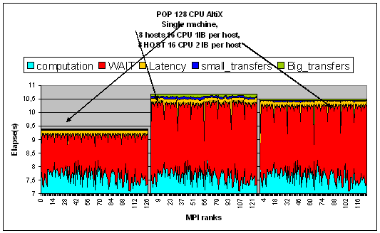
This charts shows the sensitivity of Pop (Parallel Ocean Program) to the Latency(0) of the Mpi engine.

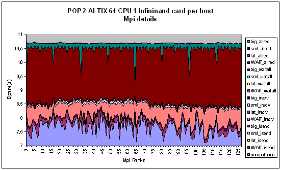
Details show that the Latency sensitivity is mainly a concern for the mpi_allreduce calls

Miscellaneous utilities

Formating the bandela.xx files:

BANDELA_ROOT/UTILS/format_event <rank> [internal]

[internal] is for debugging purpose and can be used if the BANDELA_RECORD_COMM_TIME was use during the experimentation process in order to produce the bl_comm.xx files.

Example: BANDELA_ROOT/UTILS/format_event 0

-----------Formatted rank 0 Trace-----------

Following a comcrea function : ranks of this communicator

ord: Ordinal

in: Index for ignore collective

info: request(MPI_Wait)

Short record...:

rank odi in main_f func info time

Long record....:

rank odi in main_f func comm dest tag count request time

0 1 0 init init 0 2 1009 1 4d64928d 0.000000

0 -1 0 carcrea irecv 1 1 -4 12 1 0.000000

0 -1 0 carcrea wait 1 0.000092

0 -1 0 carcrea isend 1 1 -3 24 0 0.000014

0 -1 0 carcrea wait 0 0.000018

0 -1 0 carcrea isend 1 1 -3 4 0 0.000000

0 -1 0 carcrea wait 0 0.000006

0 1 0 bcast isend 1 1 -3 8 0 0.000000

0 1 0 bcast wait 0 0.000096

0 -1 0 comcrea irecv 1 1 -4 12 1 0.000000

0 -1 0 comcrea wait 1 0.000019

0 -1 0 comcrea isend 1 1 -3 24 0 0.000001

0 -1 0 comcrea wait 0 0.000001

0 -1 0 comcrea isend 1 1 -3 4 0 0.000000

Merge the details into one column

BANDELA_ROOT/1009/UTILS/merge_column

This is a very simpleawk script which gather the four columns of the Mpi details from the column_data file into a format better suitable to be compare with the Bandelalight measurements.

Usage:

/store/dthomas/BANDELA/1005/UTILS/merge_column <column_data

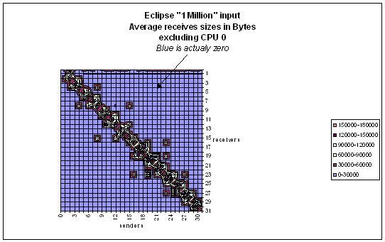
Matrix of receive sizes.

/store/dthomas/BANDELA/1005/REPLAY_SNIA/replaysend_recv < \

valid_bandela_numaflex_input

valid_bandela_numaflex_input is a valid Bandela input with Host_type=1 (numaflex).

In such case the model will works as an host_type=0 with only peak bandwidth and latency(0) being honored.

In addition you will get on a “Transfer_matrices.txt” file It contains 3 matrices, N CPU column x N CPU lines of

-Number of internal recived requests

-Total Mbytes transferred

-Average transfer size per request

Any of this matrix is intended to be looked using a spreadsheet ( An array 128x128 for example is unreadable with a text editor)

Here is an example for the average size:

Advance features

What if I optimize the computation of some routines : Caliper usage

Consider the following Fortran program

………….

call sub1()

……….

end

subroutine sub1()

……..

call sub2()

……..

return

You anticipate to reduce the CPU time of sub1 by 1.3 and the computation of sub2 by 2.

What will happen at the end is very unpredictable with an Mpi application the CPU. What you just save may be wasted waiting for an other CPU. If the Bandela traces are taken with Calipers the model can precisely respond to this question The application must be change this way:

………….

Call Bandela_caliper(5,0)

………….

call sub1()

………….

Call Bandela_caliper(0,0)

……….

End

subroutine sub1()

……..

Call Bandela_caliper(2,0)

call sub2()

Call Bandela_caliper(0,0)

……..

end

Then with the following Bandela Input :

…….

Block_max_calipers 5

Calipers_boots 1. 2. 1. 1. 1.3

……….

You will get what your optimization will bring.

Note that the following bandela input makes the model to work as if no caliper was present in the traces:

…….

Block_max_calipers 5

Calipers_boots 1. 1. 1. 1. 1.

……….

The second parameter of the Bandela_caliper routine has no meaning yet. The first argument is a caliper index. Calling bandela_caliper(0,0) unstack the previous caliper index selection. You need to define as much calipers as used by the Bandela_caliper() subrotuine in the application

What if I get ride of a synchronization point

I have some idea to avoid some synchronization points “what if” at the end

Call bandela_ignore_next_col(2,0)

Call Mpi_bcast(….

…………………

……………..

…………..

Call bandela_ignore_next_col(2,0)

Call Mpi_allreduce(….

………

……

Call bandela_ignore_next_col(1,0)

Call Mpi_barrier(….

With the following Bandela input :

…..

block_max_ignore_collective 2

# default for ignore_safely=Y

ignore_safely N

ignore_ index 1 0

With this input the Mpi_barrier will be ignored but not the Mpi_bcast or Mpi_reduce.

A call to bandela_ignore_next_col is acting only 1 time for the next Mpi routine encountered. If this routine is not a collective routine and if ignore_safely=N the model will stops. If ignore_safely=Y and if the corresponding index is set to 0, the model will continue as if no call to bandela_ignore_next_col happened.

A good Bandela usage

Don’t forget to set MPI_BUFFER_MAX accordingly for a reference run and model.

Use a “good” reference run. A one which doesn’t run into lack of data or msg buffers, a run well placed, a run where CPU computation, CPU timings change very few from one run to the other.

The input parameters given in the templates may have to be adapted to a particular situation but in most cases Bandela is VERY precise to rebuild the communication of a GOOD run occurring on an Single Altix (less than 1% error) using the input values displayed above (a copy of them are in the BANDELA_ROOT/templates directory). In case the model disagrees with the measurements do not suspect the model but suspects the run, If running with MPT checks for retries with the MPI_STATS facility for example. The model gives the conceptual numbers that the application may produce with a communication engine running correctly. If the model disagrees with reality there are something wrong occurring in the Hardware/MPI library pair that worth to investigate. Somehow we can dare to say that “the model is more accurate than reality”.

Vampir Trace generation.

-The model “replaympi” is able to generate a trace file ( trace.vpt) which could be latter viewed using The Pallas Vampir Browser. Vampirtrace generates a trace suitable for the Vampir Browser based on measurements of the Mpi communication times . Bandela (replaympi) generates a compatible trace but with the MPI communication times modeled. This is an Ascii trace, we would advise to convert it to binary trace in an independent step using the standard Vampir pvmerge utility.

No trace are generated by default.

replaympi [-s start_time] [-e end_time] [-c pico_second_clok ][-v]<input_paramaters

-v activates the the Vampir trace generation. -s and –e are ignore if –v is not set. –v creates a file trace.vpt

-If set the start time is just an indication. The trace will only start when and if an mpi_barrier is encountered.

-c change the Vampir clock resolution default value is 0.8 Microsecond. I.e. -c800000

Bandelalight.

In the same directory than libbandela.so/libbandela.a one can find libbandelalight.so/libbandelallight.a. This is a (light ) low overhead library that collects (measures) statistics related to the MPI communications.

Environment variables recognized by Libbandelalight:

Select a Window:

BANDELA_WATCH_ROUT

BANDELA_BARRIER_START

BANDELA_BARRIER_END

BANDELA_COMM_T_W

Interval to print the number of calls to the selected routine:

BANDELA_SHOW_W

This allows to select the same window of observation for communication measurement (libbandelalight) and for modeling (libbandela) and this is the better way for checking the accuracy of the model.

At the end of the run a file: bandela_stats is created. Here is an example for a 4 CPU run.

>>>> Receive Matrix (Mb) <<<<

Receive Matrix (Mb) <<<<

Lines are receivers , columns are senders

CPU 0 1 2 3

0 0.000 57.243 25.693 0.517

1 87.842 0.000 0.610 25.972

2 61.848 0.495 0.000 37.043

rank 0 Bytes buffered= 73.789 MBytes, internal send/recv requests=86091, total Barrier requests=2

rank 1 Bytes buffered= 80.692 MBytes, internal send/recv requests=87735, total Barrier requests=2

rank 2 Bytes buffered= 59.409 MBytes, internal send/recv requests=66148, total Barrier requests=2

rank 3 Bytes buffered= 63.250 MBytes, internal send/recv requests=69943, total Barrier requests=2

>>>> Request times in seconds <<<<

Time transfering is computed based of 700.000000 MB/s Bandwidth. This time not only

take into account the above recv but also includes time for buffering sends.

Such buffering as well as local recv are computed using double Bandwidth

Latency time is computed based of 2.000000 Micro second per internal send/recv request.

Barrier Latency time is computed based of 10.000000 Micro second per MPI_Barrier request.

CPU Comput Wait Latency Transfer send ...... barrier wait allreduc reduce allgathe gather

0000 273.1785 65.9074 0.1722 0.1719 0.4147 ...... 0.0048 20.2849 28.1839 0.9209 0.0007 1.4254

0001 255.7327 83.3007 0.1755 0.2211 0.8133 ...... 0.0049 21.7696 44.9627 0.0209 0.0006 0.0003

0002 255.0448 84.0686 0.1323 0.1844 0.6910 ...... 0.0044 22.7878 45.9924 0.6450 0.0007 0.0003

0003 267.3547 71.7532 0.1399 0.1821 0.7509 ...... 0.0046 21.2961 37.5431 0.0345 0.0002 0.0003

>>>> Number of requests <<<<

CPU Comput Wait Latency Transfer send ...... barrier wait allreduc reduce allgathe gather

0000 ------ ---- ------- -------- 23789 ...... 10 10083 2033 88 4 3

0001 ------ ---- ------- -------- 39562 ...... 10 10083 2033 88 4 3

0002 ------ ---- ------- -------- 25725 ...... 10 10083 2033 88 4 3

0003 ------ ---- ------- -------- 35603 ...... 10 10083 2033 88 4 3

The Receive Matrix array displays the data received (this has the same format as what you can get with libandela/replaysend_recv). This include what was received following an explicit MPI_IRECV or MPI_RECV call by the user but it also includes the hidden calls issued by the MPI library for collective routines.

The following heuristic is used to compute Bytes buffered : The library assumes that any data is symmetric. So Buffering send only depends on the MPI_BUFFER_MAX value. Sends issued by some collective routines are considered sent single copy whatever the size.

In the last 2 arrays, except for Wait, Latency, Transfer, the number displayed are strictly measurement of the computations and the communications for the observed window.

Transfer : is an evaluation of the time the hardware was indeed transferring something. This is computed based of the information displayed in the first array and by using the Bandwidth defined by the BANDELA_BANDWIDTH variables.

Latency is computed based on the numbers internal send/recv/barrier requests and the values of the BANDELA_LATENCY and BANDELA_BARRIER_LATENCY variables.

Wait: is the sum of the measured communications minus the above Transfer and Latency. It gives an approximation of the time the application cannot do anything else but wait.

For a pair of GOOD runs this three numbers must be equivalent with the ones computed by the model with the following input keywords:

INTRA_HOST_BANDWIDTH_PEAK 700.

INTRA_HOST_LATENCY 2.0

INTRA_HOST_BARRIER_LATENCY 10.00

Bandelalight just use a lighter way to get them but it doesn’t allow any “What If” games.

In case you wish to apply an other latency/bandwidth definition to exploit the data MEASURED to compute the transfer-Latency-Wait describe above this simple script does it for you:

BANDELA_ROOT/UTILS/comp_latr Bandwidth_MB/s Latency_micro_s \

Barrier_latency_micro_s [PATH to bandela_stats file]

Additionally you can see how the computation/communication ratio changes in time

BANDELA_HEART_BEAT integer_heart_beat

Computation elapse times and communication elapse times are written for each CPU on bandela.(mpi_rank + 177) each integer_heart_beat call of the watched routine. The utility format_trace ( Example : format_trace 0) will generate the following output:

call Computation communication

1000 207.1109768000027 52.29531520000086

1500 207.0920743998927 54.68045520002019

2000 207.1742191999331 51.77246160000016

2500 207.1877143999957 51.36017680002058

3000 207.2967560000152 51.97978720000788

3500 207.3676232000030 51.44490240000459

4000 207.4347855999872 51.15051600004426

…………………………………………….

Each line in this example corresponds to the computation and communication time in second to reach 500 calls of the watched routine.